Microsoft Excel remains the undisputed champion of data processing, but it’s the right commands and formulas that turn a simple spreadsheet into a powerful analytical tool. Whether you’re a student, a business analyst, or just trying to organize your life, mastering a few core functions can save you countless hours of manual work.
This guide breaks down the essential Excel commands and formulas you need to transform your data management skills.
The Data Cleanup Crew: Essential Text and Data Functions
Before you analyze, you must clean. Messy data—extra spaces, inconsistent capitalization, or merged cells—can derail any analysis.
1. TRIM and CLEAN for Tidiness

- TRIM: Removes all extra spaces from text except for single spaces between words. This is vital for cleaning data imported from other sources.
- Formula: =TRIM(A1)
- CLEAN: Removes non-printable characters often imported from web pages or external systems.
2. CONCAT (or CONCATENATE/TEXTJOIN) for Combination
Combine data from multiple cells into one. This is perfect for merging first and last names or creating a full address string.
- CONCAT: The modern, simpler function for combining text.
- Formula: =CONCAT(A1, ” “, B1) (Combines A1, a space, and B2)
- TEXTJOIN: An even more powerful option that lets you specify a delimiter (like a comma or a space) and easily ignore empty cells across a range.
3. LEFT, RIGHT, and MID for Extraction
These functions allow you to slice and dice text strings to pull out specific parts, like area codes from phone numbers or product codes from descriptions.
- LEFT: Extracts a specified number of characters from the start of a text string.
- Formula: =LEFT(A1, 3) (Pulls the first 3 characters)
- RIGHT: Extracts a specified number of characters from the end of a text string.
- MID: Extracts characters starting from a specified position and continuing for a specified length.
The Analytical Powerhouses: Conditional Formulas
These formulas allow you to perform calculations or counts based on specific criteria, giving you powerful summaries from large datasets.

1. IF for Logical Decisions
The fundamental decision-maker in Excel. It checks if a condition is true, then returns one value if true, and a different value if false.
- Formula: =IF(A1>100, “High”, “Low”)
- Use Case: Automatically assign a “Pass” or “Fail” status based on a test score.
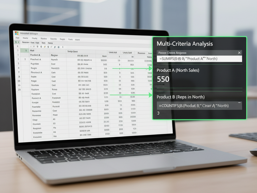
2. SUMIFS and COUNTIFS for Multi-Criteria Aggregation
If SUM and COUNT are basic, the “IFS” functions are advanced. They are crucial for filtering and summarizing data.

- SUMIFS: Sums values in a range that meet multiple criteria.
- Example: Summing sales for “Product X” only in the “North” region.
- COUNTIFS: Counts the number of cells in a range that meet multiple criteria.
- Example: Counting how many employees in the “Marketing” department have a salary above $50,000.
3. AVERAGEIFS
Similar to SUMIFS, this function calculates the average of values in a range that meet multiple criteria.
- Example: Finding the average test score for all female students in the 10th grade.
The Lookup Masters: Finding and Linking Data
No more manually searching for corresponding data in a massive table. Lookup functions automate the process of linking data between sheets or tables.
1. XLOOKUP (The Modern Standard)
XLOOKUP is the successor to VLOOKUP and HLOOKUP. It’s simpler, more flexible, and can look up values to the left (a major VLOOKUP limitation).
- What it does: Searches a range for a value and returns the corresponding value from a second range.
- Formula: =XLOOKUP(lookup_value, lookup_array, return_array)
- Use Case: Look up an employee’s name (the return_array) based on their Employee ID (the lookup_value) in the employee data table (lookup_array).
2. IFERROR for Clean Results
When a lookup function fails to find a match, it returns an error like #N/A. IFERROR lets you specify a clean result instead.
- Formula: =IFERROR(XLOOKUP(…), “Not Found”)
- Use Case: Instead of showing #N/A, the cell displays the user-friendly text “Not Found.”
Beyond Formulas: Essential Processing Commands (Tools)
Formulas are great, but sometimes you need a one-time command to process a large block of data.
| Command/Tool | Tab | Purpose |
| Sort & Filter | Data | Quickly reorganize (sort) data or display only rows that meet specific criteria (filter). Filter shortcuts: Ctrl + Shift + L |
| Text to Columns | Data | Splits the contents of one column into two or more columns based on a delimiter (like a comma or space) or a fixed width. |
| Remove Duplicates | Data | A quick-click tool to delete entire duplicate rows from your dataset, leaving only unique records. |
| PivotTables | Insert | The ultimate summarization tool. It allows you to drag-and-drop to quickly aggregate, summarize, and reorganize large datasets without using formulas. |
| Conditional Formatting | Home | Visually applies formatting (colors, icons) to cells based on their content, making trends, outliers, or warnings instantly visible. |
